Content Preview

Lorem ipsum dolor sit amet, consectetur adipisicing elit. Odit molestiae mollitia laudantium assumenda nam eaque, excepturi, soluta, perspiciatis cupiditate sapiente, adipisci quaerat odio voluptates consectetur nulla eveniet iure vitae quibusdam? Excepturi aliquam in iure, repellat, fugiat illum voluptate repellendus blanditiis veritatis ducimus ad ipsa quisquam, commodi vel necessitatibus, harum quos a dignissimos.

Keyboard Shortcuts

Help F1 or ? Previous Page ← + CTRL (Windows) ← + ⌘ (Mac) Next Page → + CTRL (Windows) → + ⌘ (Mac) Search Site CTRL + SHIFT + F (Windows) ⌘ + ⇧ + F (Mac) Close Message ESC

9.2.3 - Assumptions for the SLR Model

In this section, we will present the assumptions needed to perform the hypothesis test for the population slope:

\(H_0\colon \ \beta_1=0\)
\(H_a\colon \ \beta_1\ne0\)

We will also demonstrate how to verify if they are satisfied. To verify the assumptions, you must run the analysis in Minitab first.

Assumptions for Simple Linear Regression Section

1. Linearity: The relationship between \(X\) and \(Y\) must be linear. Check this assumption by examining a scatterplot of x and y.
2. Independence of errors: There is not a relationship between the residuals and the \(Y\) variable; in other words, \(Y\) is independent of errors. Check this assumption by examining a scatterplot of “residuals versus fits”; the correlation should be approximately 0. In other words, there should not look like there is a relationship.
3. Normality of errors: The residuals must be approximately normally distributed. Check this assumption by examining a normal probability plot; the observations should be near the line. You can also examine a histogram of the residuals; it should be approximately normally distributed.
4. Equal variances: The variance of the residuals is the same for all values of \(X\). Check this assumption by examining the scatterplot of “residuals versus fits”; the variance of the residuals should be the same across all values of the x-axis. If the plot shows a pattern (e.g., bowtie or megaphone shape), then variances are not consistent, and this assumption has not been met.

Example 9-4: Student height and weight (SLR Assumptions) Section

Recall that we would like to see if height is a significant linear predictor of weight. Check the assumptions required for simple linear regression.

The data can be found here university_ht_wt.txt.

The first three observations are:

To check the assumptions, we need to run the model in Minitab.

Using Minitab to Fit a Regression Model

To find the regression model using Minitab.

1. To check linearity create the fitted line plot by choosing STAT > Regression > Fitted Line Plot .
2. For the other assumptions run the regression model. Select Stat > Regression > Regression > Fit Regression Model
3. In the 'Response' box, specify the desired response variable.
4. In the 'Continuous Predictors' box, specify the desired predictor variable.
5. Click Graphs .
6. In 'Residuals plots', choose 'Four in one.'
7. Select OK .

Note! Of the 'four in one' graphs, you will only need the Normal Probability Plot, and the Versus Fits graphs to check the assumptions 2-4.

The basic regression analysis output is displayed in the session window. But we will only focus on the graphs at this point.

The graphs produced allow us to check our assumptions.

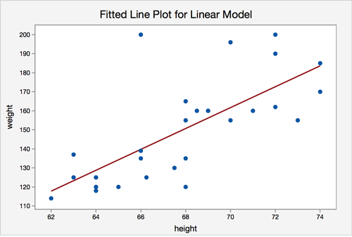
Assumption 1: Linearity - The relationship between height and weight must be linear.

The scatterplot shows that, in general, as height increases, weight increases. There does not appear to be any clear violation that the relationship is not linear.

Assumption 2: Independence of errors - There is not a relationship between the residuals and weight.

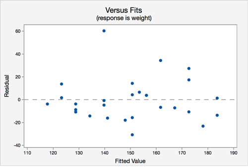
In the residuals versus fits plot, the points seem randomly scattered, and it does not appear that there is a relationship.

Assumption 3: Normality of errors - The residuals must be approximately normally distributed.

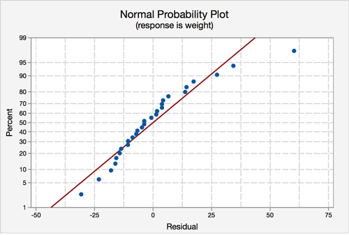
Most of the data points fall close to the line, but there does appear to be a slight curving. There is one data point that stands out.

Assumption 4: Equal Variances - The variance of the residuals is the same for all values of \(X\).

In this plot, there does not seem to be a pattern.

All of the assumption except for the normal assumption seem valid.